www.oreilly.com/library/view/hands-on-machine-learning/9781492032632/
Hands-On Machine Learning with Scikit-Learn, Keras, and TensorFlow, 2nd Edition
Through a series of recent breakthroughs, deep learning has boosted the entire field of machine learning. Now, even programmers who know close to nothing about this technology can use simple, … - Selection from Hands-On Machine Learning with Scikit-Learn
www.oreilly.com
12 장 텐서플로를 사용한 사용자 정의 모델과 훈련
사실, 앞으로 만나게 될 딥러닝 작업의 95% tf.keras 외에 다른것은 필요하지 않다.
하지만 이제 텐서플로를 자세히 들여다보고 저수준 파이썬 API를 살펴본다.
자신만의 손실 함수, 지표, 층, 모델, 초기화, 규제, 가중치 규제 등 세부적인 제어가 필요할수 있기 때문이다.
텐서플로 훑어 보기
텐서플로는 강력한 수치 계산용 라이브러리,
대규모 머신러닝에 잘맞도록 튜닝
- 넘파이와 비슷하지만 gpu 지원
- JIT(just in time) 컴파일러 포함. 속도를 높이고 메모리 사용량을 줄이기 위해 계산을 최적화 함
- 계산 그래프를 추출, 최적화(가지치기), 효율적인 실행(병렬 실행)
- 플랫폼 중립적인 포맷을 보낼 수 있어 모델 훈련과 실행이 다른 환경에서도 실행 가능
- 자동 미분, 고성능 옵티마이저를 제공하므로 손실함수를 쉽게 최소화 할 수 있음
operation은 C++ 코드로 구현되어 있음
많은 연산은 kernel이라 부르는 구현을 가짐.
각 커널은 CPU, GPU, TPU 와 같은 특정 장치에 맞추어 만들어 져 있음.
GPU는 계산을 작은 단위로 나누어 GPU 스레드에서 병렬로 실행하므로 속도를 극적으로 향상시킴.
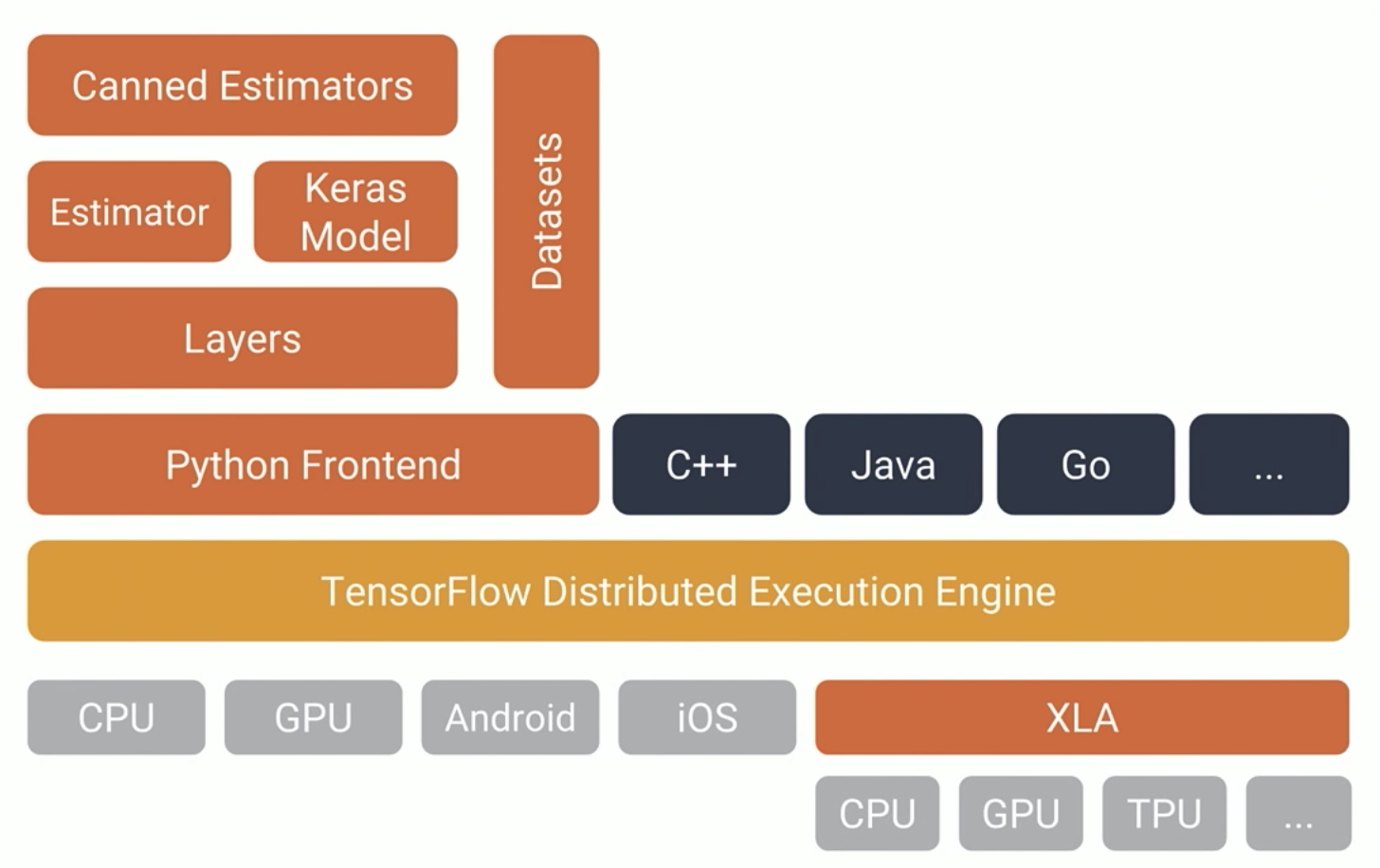
텐서플로는 하나의 라이브러리 그 이상이며 광범위한 라이브러리 생태계를 가지고 있다.
넘파이처럼 텐서플로 사용하기
텐서플로 API 는 텐서를 순환시킨다. 텐서는 한 연산에서 다른 연산으로 흐른다. (tensor-flow)
텐서는 넘파이 ndarray와 매우 비슷하다. 즉, 텐서는 다차원 배열. 스칼라 값도 가질 수 있다.
텐서와 연산
tf.constant() 함수로 텐서를 만들 수 있다.
두개의 행과 세개의 열을 가진 실수를 가진 행렬 생성
tf.constant([[1., 2., 3.], [4., 5., 6.]]) # 행렬
# <tf.Tensor: shape=(2, 3), dtype=float32, numpy=
# array([[1., 2., 3.],
#       [4., 5., 6.]], dtype=float32)>
스칼라 값도 생성 가능
tf.constant(42) # 스칼라
# <tf.Tensor: shape=(), dtype=int32, numpy=42>
ndarray와 마찬가지로 shape과 dtype을 가짐
t = tf.constant([[1., 2., 3.], [4., 5., 6.]])

t.shape() # TensorShape([2,3])

t.dtype() # tf.float32
인덱스 참조도 비슷
t[:, 1:]
#<tf.Tensor: shape=(2, 2), dtype=float32, numpy=
# array([[2., 3.],
#       [5., 6.]], dtype=float32)>
모든 종류의 텐서 연산이 가능
t + 10
# <tf.Tensor: shape=(2, 3), dtype=float32, numpy=
# array([[11., 12., 13.],
#       [14., 15., 16.]], dtype=float32)>
tf.square(t)
# <tf.Tensor: shape=(2, 3), dtype=float32, numpy=
# array([[ 1.,  4.,  9.],
#       [16., 25., 36.]], dtype=float32)>

t @ tf.transpose(t)
# <tf.Tensor: shape=(2, 2), dtype=float32, numpy=
# array([[14., 32.],
#       [32., 77.]], dtype=float32)>
필요한 모든 기본 수학 연산
- add
- multiply
- square
- exp
- sqrt
넘파이에서 볼수있는 대부분의 연산
- reshape
- squeeze
- title
을 제공함.
일부 함수는 이름이 다른데 , 다른 이유가 있음
텐서플로에서는 전치된 데이터의 복사본으로 새로운 텐서가 만들어지지만, 넘파이에서 t.T는 동일 데이터의 전치된 뷰일 뿐이다.
tf.reduce_sum() 연산은 gpu 커널이 원소가 추가된 순서를 보장하지 않는 reduce 알고리즘을 사용하기 때문, reduce_mean()도 마찬가지
텐서와 넘파이
넘파이 배열과 <-> 텐서 는 각자 서로를 이용해 만들수 있음
a = np.array([2., 4., 5.])
tf.constant(a)
# <tf.Tensor: shape=(3,), dtype=float64, numpy=array([2., 4., 5.])>
t.numpy()
# array([[1., 2., 3.],
# [4., 5., 6.]], dtype=float32)np.array(t)
# array([[1., 2., 3.],
# [4., 5., 6.]], dtype=float32)tf.square(a)
# <tf.Tensor: shape=(3,), dtype=float64, numpy=array([ 4., 16., 25.])>np.square(t)
# array([[ 1., 4., 9.],
# [16., 25., 36.]], dtype=float32)넘파이는 기본 64 bit 정밀도, 텐서플로는 32bit 정밀도 사용
타입 변환
타입 변환은 성능을 크게 감소 시킬 수 있음
타입이 자동으로 변환되면 사용자가 눈치재지 못할 수 있기 때문에, 이를 방지하고자 텐서플로는 어떤 변환도 자동으로 수행하지 않음.
예를 들어 32비트 실수와 64 비트 실수를 더할 수 없음
try:
    tf.constant(2.0) + tf.constant(40., dtype=tf.float64)
except tf.errors.InvalidArgumentError as ex:
    print(ex)

# cannot compute AddV2 as input #1(zero-based) was expected to be a float tensor but is a double tensor [Op:AddV2]
타입 변환이 정말 필요할때는 Cast 가능
t2 = tf.constant(40., dtype=tf.float64)
tf.constant(2.0) + tf.cast(t2, tf.float32)
변수
tf.constant로 생성한 Tensor는 변경이 불가능한 객체
변경이 가능한 텐서를 만들고 싶을 땐, tf.Variable로 변수 생성 가능
v = tf.Variable([[1., 2., 3.], [4., 5., 6.]])assign 메서드를 통해 변수 값을 바꿀 수 있음
v.assign(2 * v)
# array([[ 2.,  4.,  6.],
#       [ 8., 10., 12.]], dtype=float32)>

v[0, 1].assign(42)

# <tf.Variable 'UnreadVariable' shape=(2, 3) dtype=float32, numpy=
# array([[ 2., 42.,  6.],
# [ 8., 10., 12.]], dtype=float32)>

v[:, 2].assign([0., 1.])

v.scatter_nd_update(indices=[[0, 0], [1, 2]],
                    updates=[100., 200.])
# <tf.Variable 'UnreadVariable' shape=(2, 3) dtype=float32, numpy=
# array([[100.,  42.,   0.],
#       [  8.,  10., 200.]], dtype=float32)>
다른 데이터 구조
텐스 플로는 다음과 같이 몇가지 다른 데이터 구조도 지원함
- 희소 텐서 sparse tensor
- 대부분 0으로 채워진 텐서를 효율적으로 나타냄
- 텐서 배열 tensor array
- 텐서의 리스트, 리스트에 포함된 텐서는 같은 타입, 크기를 가지고 있어야함
- 래그드 텐서 ragged tensor
- 리스트의 리스트, 타입은 같아야 하지만, 각 리스트의 길이는 다를 수 있음
- 문자열 텐서 string tensor
- 유니코드가 아닌 바이트 문자열, 유니코드 문자열 사용시 utf8로 인코딩됨
- 집합 set
- 집합은 일반적인 텐서로 나타냄. eg.) tf.constant([[1,2],[3,4]])는 두개의 집합 {1, 2} 와 {3,4} 를 나타냄
- 큐 queue
- 큐는 단계별로 텐서를 저장함 FIFO
- Priorty Queue, Random ShuffleQueue, PadingFIFOQueue 등을 지원
사용자 정의 모델과 훈련 알고리즘
가장 많이 사용하는 사용자 손실 함수를 만들어 봅시다
사용자 손실 함수
손실 함수 중 평균 제곱 오차를 사용할 경우 이상치에 대해 과한 벌칙을 가하기 때문에 정확하지 않은 모델을 만들어 냄
후버 손실을 사용하면 좋은 대안책이 됨.
Huber
오차가 임계값보다 작을때 이차 함수, 임계값 보다 크면 선형 함수
선형 함수 부분은 평균 제곱오차보다 이상치에 덜 민감함
이차 함수 부분은 평균 절대값 오차보다 더빠르고 정확하게 수렴하도록 도와줌
def huber_fn(y_true, y_pred):
    error = y_true - y_pred
    is_small_error = tf.abs(error) < 1
    squared_loss = tf.square(error) / 2
    linear_loss = tf.abs(error) - 0.5
    return tf.where(is_small_error, squared_loss, linear_loss)
tf.where
Return the elements where condition is True (multiplexing x and y).
tf.where([True, False, False, True], [1,2,3,4], [100,200,300,400])

# [1, 200, 300, 4]
model.complie(loss=huber_fn, optimizer="nadam")
model.fit(X_train, y_tain, [...])사용자 정의 요소를 가진 모델을 저장하고 로드하기
케라스가 함수이름을 저장하므로 손실함수를 사용하는 모델은 아무 이상없이 저장됨
모델 로드시 함수 이름과 실제 함수를 매핑한 딕셔너리를 전달해야함
model.save("my_model_with_a_custom_loss.h5")

model = keras.models.load_model("my_model_with_a_custom_loss.h5",
                                custom_objects={"huber_fn": huber_fn})
다른 기준을 가진 huber 손실 함수 만들기
def create_huber(threshold=1.0):
    def huber_fn(y_true, y_pred):
        error = y_true - y_pred
        is_small_error = tf.abs(error) < threshold
        squared_loss = tf.square(error) / 2
        linear_loss  = threshold * tf.abs(error) - threshold**2 / 2
        return tf.where(is_small_error, squared_loss, linear_loss)
    return huber_fn
모델 저장시 threshold 값은 저장되지 않으므로
모델을 로드할때 threashhold 값을 지정해주어야함
model = keras.models.load_model("my_model_with_a_custom_loss_threshold_2.h5",
                                custom_objects={"huber_fn": create_huber(2.0)})
class HuberLoss(keras.losses.Loss):
def __init__(self, threshold=1.0, **kwargs):
self.threshold = threshold
super().__init__(**kwargs)
def call(self, y_true, y_pred):
error = y_true - y_pred
is_small_error = tf.abs(error) < self.threshold
squared_loss = tf.square(error) / 2
linear_loss = self.threshold * tf.abs(error) - self.threshold**2 / 2
return tf.where(is_small_error, squared_loss, linear_loss)
def get_config(self):
base_config = super().get_config()
return {**base_config, "threshold": self.threshold}model = keras.models.Sequential([
keras.layers.Dense(30, activation="selu", kernel_initializer="lecun_normal",
input_shape=input_shape),
keras.layers.Dense(1),
])
model.compile(loss=HuberLoss(2.), optimizer="nadam", metrics=["mae"])모델을 저장 할 때 케라스는 손실 객체의 get_config() 메서드를 호출하여 반환된 설정을 HDF5 파일에 json 형태로 저장
모델 로드시 HuberLoss Class의 from_config() 메서드를 호출해 생성자에게 **config 매개변수를 전달해 클래스의 인스턴스를 만듬
활성화 함수, 초기화, 규제, 제한을 커스터마이징 하기
손실, 규제, 제한, 초기화, 지표, 활성화 함수, 층, 모델 등 대부분의 케라스 기능은 유사한 방법으로 커스터마이징 할 수 있다.
대부분의 경우 적절한 입력과 출력을 가진 간단한 함수를 작성하면 됨
사용자 정의 활성화 함수, 초기화 함수, 규제, 제한 예시
def my_softplus(z): # tf.nn.softplus(z) 값을 반환합니다
    return tf.math.log(tf.exp(z) + 1.0)

def my_glorot_initializer(shape, dtype=tf.float32):
    stddev = tf.sqrt(2. / (shape[0] + shape[1]))
    return tf.random.normal(shape, stddev=stddev, dtype=dtype)

def my_l1_regularizer(weights):
    return tf.reduce_sum(tf.abs(0.01 * weights))

def my_positive_weights(weights): # tf.nn.relu(weights) 값을 반환합니다
    return tf.where(weights < 0., tf.zeros_like(weights), weights)
# Creates a tensor with all elements set to zero.
tensor = tf.constant([[1, 2, 3], [4, 5, 6]])
tf.zeros_like(tensor)
# [[0,0,0,], [0,0,0]]위의 예시에서 알 수 있듯 매개 변수는 함수의 종류에 따라 다르다.
layer = keras.layers.Dense(1, activation=my_softplus,
                           kernel_initializer=my_glorot_initializer,
                           kernel_regularizer=my_l1_regularizer,
kernel_constraint=my_positive_weights)- 활성화 함수는 Dense 출력층에 적용
- 가중치는 초기화 함수에서 반환된 값으로 초기화
- 훈련 스텝마다 가중치가 규제 함수에 전달되어 규제 손실 계산하여, 전체 손실에 추가 되어 최종 손실을 만듬
- 제한 함수가 훈련 스텝마다 층의 가중치를 제한한 가중치 값으로 바꿈
함수가 모델과 함께 저장해야 할하이퍼 파라미터를 가지고 있다면
- keras.regularizers.Regularizer
- keras.constraints.Constraint
- keras.initiazliers.Initializer
- keras.layers.Layer
적절한 클래스를 상속하여 구현
class MyL1Regularizer(keras.regularizers.Regularizer):
    def __init__(self, factor):
        self.factor = factor
    def __call__(self, weights):
        return tf.reduce_sum(tf.abs(self.factor * weights))
    def get_config(self):
        return {"factor": self.factor}
model = keras.models.Sequential([
keras.layers.Dense(30, activation="selu", kernel_initializer="lecun_normal",
input_shape=input_shape),
keras.layers.Dense(1, activation=my_softplus,
kernel_regularizer=MyL1Regularizer(0.01),
kernel_constraint=my_positive_weights,
kernel_initializer=my_glorot_initializer),
])사용자 정의 지표
손실과 지표는 개념적으로 다른것이 아님
손실
- 모델을 훈련하기위해 경사 하강법에서 사용
- 미분 가능해야하고, 그레디언트가 모든곳에서 0이 아니어야함
- 사람이 이해하기 어려워도 괜찮음
지표
- 모델을 평가할때 사용함
- 훨씬 사람이 이해하기 쉬어야 함
- 미분이 가능하지 않고, 모든곳에서 그레이디언트가 0이어도 괜찮음
대부분은 사용자 지표,손실 함수를 만드는 것은 동일함.
앞서만든 후버 손실함수도 지표로 사용해도 잘 동작함
model.compile(loss="mse", optimizer="nadam", metrics=[create_huber(2.0)])정밀도
| 배치 순서 | 예측 결과(예측성공 개수/ 전체) | 확률 |
|---|---|---|
| 1 | 4/5 | 80% |
| 2 | 0/3 | 0% |
두 정밀도의 평균은 40%
하지만 진짜 정밀도는 (4/8)50%
따라서 진짜 양성 개수와 거짓 양성 개수를 기록하고 필요시 정밀도를 계산하는 객체가 필요함
precision = keras.metrics.Precision()
precision([0, 1, 1, 1, 0, 1, 0, 1], [1, 1, 0, 1, 0, 1, 0, 1])
#<tf.Tensor: shape=(), dtype=float32, numpy=0.8>
precision([0, 1, 0, 0, 1, 0, 1, 1], [1, 0, 1, 1, 0, 0, 0, 0])
#<tf.Tensor: shape=(), dtype=float32, numpy=0.0>

precision.result()
#<tf.Tensor: shape=(), dtype=float32, numpy=0.5>

precision.variables
#[<tf.Variable 'true_positives:0' shape=(1,) dtype=float32, numpy=array([4.], dtype=float32)>,
#<tf.Variable 'false_positives:0' shape=(1,) dtype=float32, numpy=array([4.], dtype=float32)>]

precision.reset_states()
위와 같은 스트리밍 지표를 만들고 싶다면 keras.metrics.Metric 클래스를 상속받아 구현
class HuberMetric(keras.metrics.Metric):
    def __init__(self, threshold=1.0, **kwargs):
        super().__init__(**kwargs) # 기본 매개변수 처리 (예를 들면, dtype)
        self.threshold = threshold
        self.huber_fn = create_huber(threshold)
        self.total = self.add_weight("total", initializer="zeros")
        self.count = self.add_weight("count", initializer="zeros")
    def update_state(self, y_true, y_pred, sample_weight=None):
        metric = self.huber_fn(y_true, y_pred)
        self.total.assign_add(tf.reduce_sum(metric))
        self.count.assign_add(tf.cast(tf.size(y_true), tf.float32))
    def result(self):
        return self.total / self.count
    def get_config(self):
        base_config = super().get_config()
        return {**base_config, "threshold": self.threshold}
결과값을 요청하면 평균 후버 손실이 반환됨
- 생성자에서 add_weight로 기록 변수 생성
- update_state() 클래스를 함수처럼 사용할때 호출(위 precision 객체처럼)
- result() 메서드의 최종 결과를 계산하고 반환, 모든 샘플에 대한 평균 후버 손실 값
- get_config() 메서드를 구현하여 threshold 변수를 모델과 함께 저장
- reset_status() 메서드는 기본적인 모든 변수를 0.0으로 초기화함. 필요하면 함수 override 가능
사용자 정의 층
모델이 층 A,B,C,A,B,C 순서대로 구성되어 있다면
ABC를 묶어 D로 정의, D,D,D 로 구성된 모델을 만들 수 있습니다.
keras.layers.Flatten, keras.layers.ReLU 같은 층 가중치가 없습니다.
exponential_layer = keras.layers.Lambda(lambda x: tf.exp(x))상태가 있는 층(즉, 가중치)을 만드려면 keras.layers.Layer를 상속해야함
class MyDense(keras.layers.Layer):
    def __init__(self, units, activation=None, **kwargs):
        super().__init__(**kwargs)
        self.units = units
        self.activation = keras.activations.get(activation)

    def build(self, batch_input_shape):
        self.kernel = self.add_weight(
            name="kernel", shape=[batch_input_shape[-1], self.units],
            initializer="glorot_normal")
        self.bias = self.add_weight(
            name="bias", shape=[self.units], initializer="zeros")
        super().build(batch_input_shape) # must be at the end

    def call(self, X):
        return self.activation(X @ self.kernel + self.bias)

    def compute_output_shape(self, batch_input_shape):
        return tf.TensorShape(batch_input_shape.as_list()[:-1] + [self.units])

    def get_config(self):
        base_config = super().get_config()
        return {**base_config, "units": self.units,
"activation": keras.activations.serialize(self.activation)}- 생성자는 activation 문자열 매개변수를 받아 적절한 활성화 함수를 설정
- build() 메서드는 가중치마다 add_weight 함수를 호출하여 층의 변수를 만듬
- call() 메서드는 이 층에 필요한 연산을 수행
- compute_output_shape() 이 층의 출력 크기를 반환 함. 여기서는 마지막 차원을 제외하고는 입력과 크기가 같음
- get_config() 메서드는 앞서 보았던 것과 같습니다.
입력, 출력의 수를 추가하는 방법
여러가지 입력을 받는 층을 만들려면 call() 메서드에 모든 입력이 포함된 튜플을 매개변수 값으로 전달해야함
compute_output_shape() 메서드의 매개변수도 각 입력의 배치 크기를 담은 튜플이어야 함
여러 출력을 가진 층을 만들려면 call() 메서드가 출력을 반환해야함
class MyMultiLayer(keras.layers.Layer):
    def call(self, X):
        X1, X2 = X
        return X1 + X2, X1 * X2

    def compute_output_shape(self, batch_input_shape):
        batch_input_shape1, batch_input_shape2 = batch_input_shape
        return [batch_input_shape1, batch_input_shape2]
훈련과 테스트에서 다르게 동작하는 층 구현
class AddGaussianNoise(keras.layers.Layer):
    def __init__(self, stddev, **kwargs):
        super().__init__(**kwargs)
        self.stddev = stddev

    def call(self, X, training=None):
        if training:
            noise = tf.random.normal(tf.shape(X), stddev=self.stddev)
            return X + noise
        else:
            return X

    def compute_output_shape(self, batch_input_shape):
        return batch_input_shape
사용자 정의 모델
아래와 같은 그림을 가진 모델을 만들어보자

잔차 블록 정의
이 층은 다른 층을 포함하고 있음
keras는 자동으로 필요한 변수(여기서는 층)을 이층의 변수 리스트에 추가함
class ResidualBlock(keras.layers.Layer):
    def __init__(self, n_layers, n_neurons, **kwargs):
        super().__init__(**kwargs)
        self.hidden = [keras.layers.Dense(n_neurons, activation="elu",
                                          kernel_initializer="he_normal")
                       for _ in range(n_layers)]

    def call(self, inputs):
        Z = inputs
        for layer in self.hidden:
            Z = layer(Z)
        return inputs + Z
사용자 정의 정의 모델
class ResidualRegressor(keras.models.Model):
    def __init__(self, output_dim, **kwargs):
        super().__init__(**kwargs)
        self.hidden1 = keras.layers.Dense(30, activation="elu",
                                          kernel_initializer="he_normal")
        self.block1 = ResidualBlock(2, 30)
        self.block2 = ResidualBlock(2, 30)
        self.out = keras.layers.Dense(output_dim)

    def call(self, inputs):
        Z = self.hidden1(inputs)
        for _ in range(1 + 3):
            Z = self.block1(Z)
        Z = self.block2(Z)
        return self.out(Z)
생성자에서 층을 만듬, call() 메서드에서 이를 사용
이로써 시퀀셜 API, 함수형 API, 서브클래싱 API를 사용해 논문의 나오는 거의 모든 모델이나 이런 모델을 합성한 모델도 간결하게 만들 수 있음.
아직 더 살펴봐야 할것들이 있는데,
- 모델 내부 구조에 기반한 손실과 지표를 만드는 방법
- 사용자 정의 훈련 반복을 만드는 방법
모델 구성 요소에 기반한 손실과 지표
앞서 정의한 사용자 손실과 지표는 모두 레이블과 예측을 기반으로함
은닉층의 가중치나 활성화 함수 등과 같이 모델 구성 요소에 기반한 손실을 정의해야 할때가 있음
이런 손실은 모델의 내부 모니터링 상황을 모니터링 할 때 유용함
노트: TF 2.2에 있는 이슈(#46858) 때문에 build() 메서드와 함께 add_loss()를 사용할 수 없습니다. 따라서 다음 코드는 책과 다릅니다. build() 메서드 대신 생성자에 reconstruct 층을 만듭니다. 이 때문에 이 층의 유닛 개수를 하드코딩해야 합니다(또는 생성자 매개변수로 전달해야 합니다).class ReconstructingRegressor(keras.models.Model):
def __init__(self, output_dim, **kwargs):
super().__init__(**kwargs)
self.hidden = [keras.layers.Dense(30, activation="selu",
kernel_initializer="lecun_normal")
for _ in range(5)]
self.out = keras.layers.Dense(output_dim)
self.reconstruct = keras.layers.Dense(8) # TF 이슈 #46858에 대한 대책
self.reconstruction_mean = keras.metrics.Mean(name="reconstruction_error")
# TF 이슈 #46858 때문에 주석 처리
# def build(self, batch_input_shape):
# n_inputs = batch_input_shape[-1]
# self.reconstruct = keras.layers.Dense(n_inputs, name='recon')
# super().build(batch_input_shape)
def call(self, inputs, training=None):
Z = inputs
for layer in self.hidden:
Z = layer(Z)
reconstruction = self.reconstruct(Z)
self.recon_loss = 0.05 * tf.reduce_mean(tf.square(reconstruction - inputs))
if training:
result = self.reconstruction_mean(recon_loss)
self.add_metric(result)
return self.out(Z)
def train_step(self, data):
x, y = data
with tf.GradientTape() as tape:
y_pred = self(x)
loss = self.compiled_loss(y, y_pred, regularization_losses=[self.recon_loss])
gradients = tape.gradient(loss, self.trainable_variables)
self.optimizer.apply_gradients(zip(gradients, self.trainable_variables))
return {m.name: m.result() for m in self.metrics}- 생성자가 다섯개의 은닉층과 하나의 출력층으로 구성된 심층 신경망
- 생성자에서 덴스 레이어를 하나 더 추가하여 모델의 입력을 재구성하는데 사용, 완전 연결층의 유닛 개수는 입력 개수와 같아야함.
- call() 메서드에서 입력이 다섯개의 은닉층에 모두 통과시킴, 결과값을 재구성층에 넘겨 재구성 값을 만듬
- 재구성 손실을 계산하고, add_metric 함수를 호출해 모델에 지표를 추가함
- 출력층에 결과를 반환함
- train_step 마다 손실을 계산, fit에서 내부적으로 일어나는 훈련 스텝을 customize 하는 방법
- regularization_losses: Additional losses to be added to the total loss. link
class CustomModel(keras.Model):
    def train_step(self, data):
        # Unpack the data. Its structure depends on your model and
        # on what you pass to `fit()`.
        x, y = data

        with tf.GradientTape() as tape:
            y_pred = self(x, training=True)  # Forward pass
            # Compute the loss value
            # (the loss function is configured in `compile()`)
            loss = self.compiled_loss(y, y_pred, regularization_losses=self.losses)

        # Compute gradients
        trainable_vars = self.trainable_variables
        gradients = tape.gradient(loss, trainable_vars)
        # Update weights
        self.optimizer.apply_gradients(zip(gradients, trainable_vars))
        # Update metrics (includes the metric that tracks the loss)
        self.compiled_metrics.update_state(y, y_pred)
        # Return a dict mapping metric names to current value
        return {m.name: m.result() for m in self.metrics}
자동 미분을 사용하여 그레디언트 계산하기
def f(w1, w2):
return 3 * w1 ** 2 + 2 * w1 * w2- w1에 대한 도함수는 6*w1 +2
- w2에 대한 도함수는 2*w1
w1, w2 = 5, 3
eps = 1e-6

(f(w1 + eps, w2) - f(w1, w2)) / eps
# 36.000003007075065
(f(w1, w2 + eps) - f(w1, w2)) / eps
# 10.000000003174137
w1, w2 = tf.Variable(5.), tf.Variable(3.)
with tf.GradientTape() as tape:
z = f(w1, w2)
gradients = tape.gradient(z, [w1, w2])
gradients
# [<tf.Tensor: shape=(), dtype=float32, numpy=36.0>,
# <tf.Tensor: shape=(), dtype=float32, numpy=10.0>]메모리 절약을 위해서 tf.GradientTape에 최소한만을 담으세요
gradient 메서드 호출시 tape가 즉시 지워짐
with tf.GradientTape() as tape:
    z = f(w1, w2)

dz_dw1 = tape.gradient(z, w1)
try:
    dz_dw2 = tape.gradient(z, w2)
except RuntimeError as ex:
    print(ex)

# A non-persistent GradientTape can only be used tocompute one set of gradients (or jacobians)
with tf.GradientTape(persistent=True) as tape:
z = f(w1, w2)
dz_dw1 = tape.gradient(z, w1)
dz_dw2 = tape.gradient(z, w2) # works now!
del tapec1, c2 = tf.constant(5.), tf.constant(3.)
with tf.GradientTape() as tape:
z = f(c1, c2)
gradients = tape.gradient(z, [c1, c2])
# [None, None]with tf.GradientTape() as tape:
tape.watch(c1)
tape.watch(c2)
z = f(c1, c2)
gradients = tape.gradient(z, [c1, c2])
#[<tf.Tensor: shape=(), dtype=float32, numpy=36.0>,
# <tf.Tensor: shape=(), dtype=float32, numpy=10.0>]대부분의 경우 그레이디언트 계산은 여러값 에 대한 한값의 그레이디언트를 계산하는데에 사용
여러 손실이 포함된 벡터의 그레이디언트를 계산하면 벡터 합의 그레이디언트를 계산함
만약 개별 그레이디언트를 계산하고싶으면 jacobian(야코비) 메서드를 호출해야함
신경망의 일부분에 그레이디언트 역전파가 되지 않도록 막고싶다면, stop_graident() 메서드 사용
def f(w1, w2):
    return 3 * w1 ** 2 + tf.stop_gradient(2 * w1 * w2)

with tf.GradientTape() as tape:
    z = f(w1, w2)

tape.gradient(z, [w1, w2])
# [<tf.Tensor: shape=(), dtype=float32, numpy=30.0>, None]
가끔 그레이디언트 계산시 부동소수점 정밀도 오류로 인해 자동 미분이 무한 나누기 계산을 하게되어 NaN이 반환됨
x = tf.Variable(100.)
with tf.GradientTape() as tape:
    z = my_softplus(x)

tape.gradient(z, [x])
다행이 수치적으로 안전한 소프트플러스의 도함수를 해석적으로 구할수 있음.
@tf.custom_gradient 데코레이터를 사용하여 일반 출력과 도함수를 계산하는 함수를 반환하여 텐서플로가 my_softplus 함수의 그레이디언트를 계산할때 안전한 함수를 사용하도록 만듬
@tf.custom_gradient
def my_better_softplus(z):
    exp = tf.exp(z)
    def my_softplus_gradients(grad):
        return grad / (1 + 1 / exp)
    return tf.math.log(exp + 1), my_softplus_gradients
사용자 정의 훈련 반복
fit() 메서드의 유연성이 원하는 만큼 충분하지 않을 수 있음
사용자 훈련을 직접 만드는 것의 단점
- 길고
- 버그가 발생하기 쉽고
- 유지보수하기 어려운 코드가 만들어진다
정말로 필요한게 아니면, fit()을 사용하는것을 권장
keras.backend.clear_session()
np.random.seed(42)
tf.random.set_seed(42)
l2_reg = keras.regularizers.l2(0.05)
model = keras.models.Sequential([
keras.layers.Dense(30, activation="elu", kernel_initializer="he_normal",
kernel_regularizer=l2_reg),
keras.layers.Dense(1, kernel_regularizer=l2_reg)
])def random_batch(X, y, batch_size=32):
idx = np.random.randint(len(X), size=batch_size)
return X[idx], y[idx]def print_status_bar(iteration, total, loss, metrics=None):
metrics = " - ".join(["{}: {:.4f}".format(m.name, m.result())
for m in [loss] + (metrics or [])])
end = "" if iteration < total else "\n"
print("\r{}/{} - ".format(iteration, total) + metrics,
end=end)import time
mean_loss = keras.metrics.Mean(name="loss")
mean_square = keras.metrics.Mean(name="mean_square")
for i in range(1, 50 + 1):
loss = 1 / i
mean_loss(loss)
mean_square(i ** 2)
print_status_bar(i, 50, mean_loss, [mean_square])
time.sleep(0.05)n_epochs = 5
batch_size = 32
n_steps = len(X_train) // batch_size
optimizer = keras.optimizers.Nadam(lr=0.01)
loss_fn = keras.losses.mean_squared_error
mean_loss = keras.metrics.Mean()
metrics = [keras.metrics.MeanAbsoluteError()]for epoch in range(1, n_epochs + 1):
print("Epoch {}/{}".format(epoch, n_epochs))
for step in range(1, n_steps + 1):
X_batch, y_batch = random_batch(X_train_scaled, y_train)
with tf.GradientTape() as tape:
y_pred = model(X_batch)
main_loss = tf.reduce_mean(loss_fn(y_batch, y_pred))
loss = tf.add_n([main_loss] + model.losses)
gradients = tape.gradient(loss, model.trainable_variables)
optimizer.apply_gradients(zip(gradients, model.trainable_variables))
for variable in model.variables:
if variable.constraint is not None:
variable.assign(variable.constraint(variable))
mean_loss(loss)
for metric in metrics:
metric(y_batch, y_pred)
print_status_bar(step * batch_size, len(y_train), mean_loss, metrics)
print_status_bar(len(y_train), len(y_train), mean_loss, metrics)
for metric in [mean_loss] + metrics:
metric.reset_states()- 두개의 반복문 중첩 (에포크, 배치)
- random_batch로 랜덤하게 샘플링
- tf.GradientTape 블럭 안에서 모델을 사용하여 예측을하고, loss_fn을 통해 로스 계산, 평균을 loss를 계산, 규제 손실 loss를 더함
- 훈련가능한 각 변수의 손실에 대한 gradient계산, 경사 하강법 수행
- 모델에 가중치 제한을 두었으면 제한 적용
- 평균 손실과 지표를 업데이트 상태막대 출력
- 매 에포크 평균 손실과 지표를 초기화
텐서플로 함수와 그래프
텐서플로 1에서 그래프는 텐서플로 API의 핵심으로 피할수 없었고 복잡도가 높았음
텐서플로 2에도 그래프가 있지만, 이전만큼 핵심적이지는 않고 사용하기가 매우 쉬워짐 (그래프 자동 생성 기능 때문)
def cube(x):
    return x ** 3


cube(2)
# 8

cube(tf.constant(2.0))
# <tf.Tensor: shape=(), dtype=float32, numpy=8.0>
tf.function을 사용하면, 파이썬 함수를 텐서플로 함수로 바꿀 수 있음
tf_cube = tf.function(cube)
tf_cube
# <tensorflow.python.eager.def_function.Function at 0x7f11c88fed00>


tf_cube(2)
# <tf.Tensor: shape=(), dtype=int32, numpy=8>
tf_cube(tf.constant(2.0))
# <tf.Tensor: shape=(), dtype=float32, numpy=8.0>
원본 함수가 필요할 때
tf.cube.python_function(2)
# 8- 텐서플로는 사용하지 않는 노드를 제거하고 표현을 단수화 하여 계산 그래프를 최적화
- 가능하면 병렬로 연산을 수행하여 효율적으로 실행, 복잡한 연산을 수행할때 두드러짐
- 파이썬 함수를 빠르게 실행하려면 텐서플로 함수로 변환!
텐서플로는 입력 크기와 데이터 타입에 맞춰 새로운 그래프 를 생성하고, 다음 입력에 대해 재사용 가능한 경우 재사용, 혹은 재생성을 함
tf_cube(tf.constant(10)) # 그래프 생성
tf_cube(tf.constant(20)) # 그래프 재사용

tf_cube(tf.constant([10, 20])) # 그래프 생성
오토그래프와 트레이싱
텐서 플로가 어떻게 그래프를 생성할까?
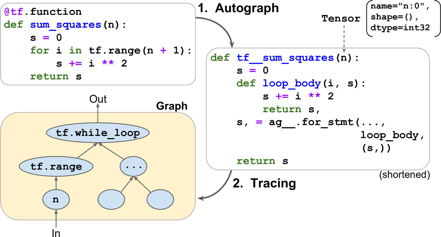
- 오토그래프
- 소스코드를 분석하여 제어문을 모두 찾음 (for,while,if, brea,continue, return)
- 이 제어문을 텐서플로 연산으로 바꿈
- while -> tf.while_loop()
- for문 블록 loop_body
- if -> tf.cond()
- 트레이싱
- 텐서플로가 업그레이드 된 함수 호출, 하지만 매개변수 값을 전달하는 대신, 심볼릭 텐서를 전달
- 심볼릭 텐서 : 실제 값이 없고, 데이터 타입, 크기만 가짐
- 트레이싱을 할때 그래프가 완성되며 같은 tf.dtype에 대해서는 한번만 실행됨
- 텐서플로가 업그레이드 된 함수 호출, 하지만 매개변수 값을 전달하는 대신, 심볼릭 텐서를 전달
텐서플로 함수 사용 방법
1. 넘파이나 표준 라이브러리 호출시 트레이싱 과정에 호출되어 그래프 연산에 포함되지 않음
이에 따라 발생하는 Effect 들이 있는데 몇가지 예시를 들면
- np.random.rand()를 사용하면, 같은 dtype input에 대해서는 같은 난수가 fix 되어 있음(그래프 내에 상수화 저장?)
- 텐서플로에서 지원하지 않는 코드, 로깅 코드라면 트레이싱시에만 실행되므로 로깅이 되지 않음
- 아무 코드나 tf.py_function을 감쌀수있지만, 하지만 텐서플로가 어떤 최적화 불가능하면 성능에 방해가 될뿐이다
2. 그래프 모드로 계산할 첫번째 함수만 데코레이터를 적용하면, 내부에서 사용하는 함수들은 감지가 되어 같은 규칙을 따름
3. 함수에서 텐서플로 변수를 만든다면, 처음에만 호출되어야 한다.
아니면 exception 발생.
변수에 값 할당시 = 연산자 대신 assign() 메서드를 사용하라
4. 파이썬 함수의 소스코드는 텐서플로에서 사용 가능해야함
Python shell에서 실행하거나, 컴파일된 *.pyc 배포시 접근 불가면, 그래프 생성 과정이 실패하거나 일부 기능을 사용 할 수 없다.
5. 텐서플로는 텐서나 데이터 셋을 순회하는 for문만 감지한다.
for i in ragne(x) 대신, for i in tf.range(x)를 사용하라
@tf.function
def add_10(x):
    for i in range(10):
        x += 1
    return x
[<tf.Operation 'x' type=Placeholder>,
<tf.Operation 'add/y' type=Const>,
<tf.Operation 'add' type=AddV2>,
<tf.Operation 'add_1/y' type=Const>,
<tf.Operation 'add_1' type=AddV2>,
<tf.Operation 'add_2/y' type=Const>,
<tf.Operation 'add_2' type=AddV2>,
<tf.Operation 'add_3/y' type=Const>,
<tf.Operation 'add_3' type=AddV2>,
<tf.Operation 'add_4/y' type=Const>,
<tf.Operation 'add_4' type=AddV2>,
<tf.Operation 'add_5/y' type=Const>,
<tf.Operation 'add_5' type=AddV2>,
<tf.Operation 'add_6/y' type=Const>,
<tf.Operation 'add_6' type=AddV2>,
<tf.Operation 'add_7/y' type=Const>,
<tf.Operation 'add_7' type=AddV2>,
<tf.Operation 'add_8/y' type=Const>,
<tf.Operation 'add_8' type=AddV2>,
<tf.Operation 'add_9/y' type=Const>,
<tf.Operation 'add_9' type=AddV2>,
<tf.Operation 'Identity' type=Identity>]
(오토그래프에 의한) tf.range()를 사용한 동적인 for 반복:
@tf.function
def add_10(x):
    for i in tf.range(10):
        x = x + 1
    return x
[<tf.Operation 'x' type=Placeholder>,
<tf.Operation 'range/start' type=Const>,
<tf.Operation 'range/limit' type=Const>,
<tf.Operation 'range/delta' type=Const>,
<tf.Operation 'range' type=Range>,
<tf.Operation 'sub' type=Sub>,
<tf.Operation 'floordiv' type=FloorDiv>,
<tf.Operation 'mod' type=FloorMod>,
<tf.Operation 'zeros_like' type=Const>,
<tf.Operation 'NotEqual' type=NotEqual>,
<tf.Operation 'Cast' type=Cast>,
<tf.Operation 'add' type=AddV2>,
<tf.Operation 'zeros_like_1' type=Const>,
<tf.Operation 'Maximum' type=Maximum>,
<tf.Operation 'while/maximum_iterations' type=Const>,
<tf.Operation 'while/loop_counter' type=Const>,
<tf.Operation 'while' type=StatelessWhile>,
<tf.Operation 'Identity' type=Identity>]6. 성능 면에서는 반복문보다 가능한 벡터화된 구현을 사용하는것이 좋다.
'프로그래밍 > AI' 카테고리의 다른 글
| msbuild-mcp-server로 C++/C# 코드 빌드 결과를 LLM Agent에 연결하기 (1) | 2025.05.07 |
|---|---|
| 케라스를 사용한 인공신경망 소개 (0) | 2021.02.02 |
| Bias and Vairance (0) | 2019.05.05 |
| Double-Dueling-dqn 분석 (0) | 2019.05.05 |
| Ubuntu Tensorflow-gpu 설치 (0) | 2019.05.05 |